Arc Institute recently unveiled the Virtual Cell Challenge. Participants are required to train a model capable of predicting the effect of silencing a gene in a (partially) unseen cell type, a task they term context generalization. For ML engineers with little to no biology background, the jargon and required context can seem quite daunting. To encourage participation, we recapitulate the challenge in a form better suited to engineers from other disciplines.

Background

Goal
Train a model to predict the effect on a cell of silencing a gene using CRISPR.

Doing things in the world of atoms is expensive, laborious and error prone. What if we could test thousands of drug candidates without ever touching a petri dish? This is the goal of the virtual cell challenge — a model (most likely a neural network) that can simulate exactly what happens to a cell when we change some parameter. Given that tightening your feedback loop is often the best way to speed up progress, a model capable of doing this accurately would have significant impact.

To train this neural network, we will need data. For the challenge, Arc has curated a dataset of ~300k single-cell RNA sequencing profiles. It may be worthwhile to revisit the Central Dogma before continuing. This essay will build off of this to provide the ~minimum biology knowledge you'll need for the challenge.

Training data

The training set consists of a sparse matrix and some associated metadata. More specifically, we have 220k cells, and for each cell we have a transcriptome. This transcriptome is a sparse row vector, where each entry is the raw count of RNA molecules (transcripts) that the corresponding gene (our column) encodes for. Of the 220k cells, ~38k are unperturbed, meaning no gene has been silenced using CRISPR. These control cells are crucial as we will see shortly.

To understand the dataset more concretely, let's select a gene, TMSB4X (the most frequently silenced gene in the dataset) and compare the number of RNA molecules detected for a control cell and a perturbed cell.

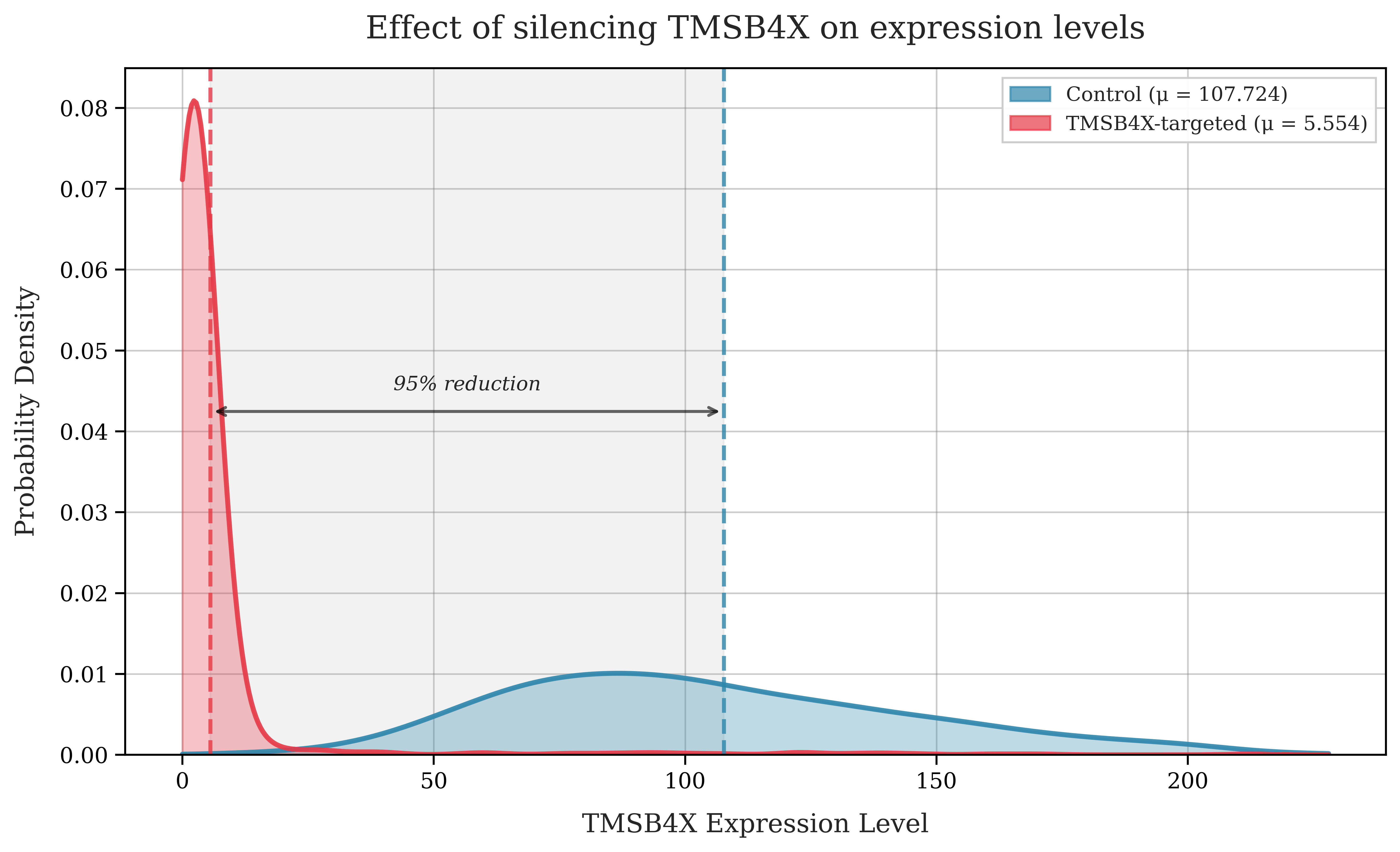
We can see that the cell with TMSB4X silenced has a greatly reduced number of transcripts compared with the control cells.

Modelling the challenge

The astute among you may be wondering why you don't just measure the count of the RNA molecules before and after silencing the gene — why do we need the control cells at all? Unfortunately, reading the transcriptome destroys the cell, which is a problem reminiscent of the observer effect.

This inability to measure the cell state before and after introduces many issues, as we are forced to use a population of basal (a.k.a control, unperturbed) cells as a reference point. The control cells and perturbed cells are not entirely homogeneous even prior to the perturbation. This means that we have to now separate out our true signal, the perturbation, from noise induced by the heterogeneity.

More formally, we can model observed gene expression in perturbed cells as:

$$\hat{X}_p \sim \hat{T}_p(\mathcal{D}_{\text{basal}}) + H(\mathcal{D}_{\text{basal}}) + \varepsilon, \quad \varepsilon \sim P_\varepsilon$$

where:

• $\hat{X}_p$: The observed gene expression measurements in cells with perturbation $p$
• $\mathcal{D}_{\text{basal}}$: The distribution of the unperturbed, baseline cell population.
• $\hat{T}_p(\mathcal{D}_{\text{basal}})$: True effect caused by perturbation $p$ on the population.
• $H(\mathcal{D}_{\text{basal}})$: Biological heterogeneity of the baseline population.
• $\varepsilon$: Experiment-specific technical noise, assumed independent of the unperturbed cell state and $\mathcal{D}_{\text{basal}}$.

STATE: The baseline from Arc

Prior to the Virtual Cell Challenge, Arc released STATE, their own attempt to solve the challenge using a pair of transformer based models. This serves as a strong baseline for participants to start with, so we will explore it in detail.

STATE consists of two models, the State Transition Model (ST) and the State Embedding Model (SE). SE is designed to produce rich semantic embeddings of cells in an effort to improve cross cell type generalization. ST is the "cell simulator", that takes in either a transcriptome of a control cell, or an embedding of a cell produced by SE, along with a one hot encoded vector representing the perturbation of interest, and outputs the perturbed transcriptome.

State Transition Model (ST)

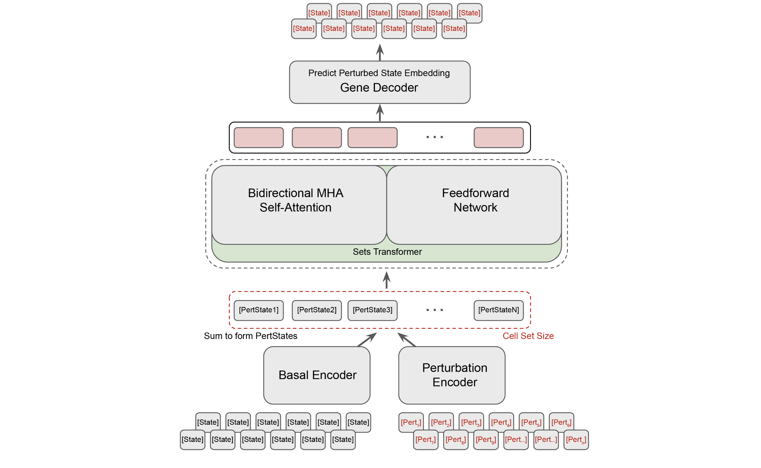
The State Transition Model is a relatively simple transformer with a Llama backbone that operates upon the following:

1. A set of transcriptomes (or SE embeddings) for covariate matched basal cells.
2. A set of one hot vectors representing our gene perturbation for each cell.

Using a covariate matched set of control cells with paired target cells should assist the model in discerning the actual effect of our intended perturbation. Both the control set tensor and the perturbation tensor are fed through independent encoders, which are simply 4 layer MLPs with GELU activations. If working directly in gene expression space (i.e producing a full transcriptome), they pass the output through a learned decoder.

ST is trained using Maximum Mean Discrepancy. Put simply, the model learns to minimize the difference between the two probability distributions.

State Embedding Model (SE)

The State Embedding Model is a BERT-like model trained using a masked prediction task. To understand this more deeply, first we have to take a little detour for some more biological grounding.

A little biological detour

A gene consists of exons (protein coding sections) and introns (non-protein coding sections). DNA is first transcribed into pre-mRNA, as shown above. The cell then performs Alternative Splicing. This is basically "pick and choose exons", cut out all introns. You can think of the gene as an IKEA manual for making a table. One could also construct a 3 legged table, perhaps an odd bookshelf with some effort, by leaving out some parts. These different objects are analogous to protein isoforms, proteins coded for by the same gene.

Back to the model

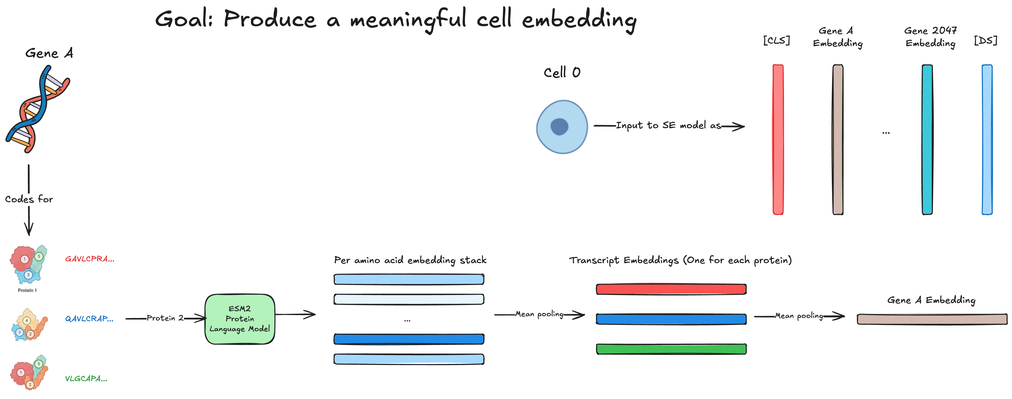
With this basic understanding, we can move on to how the SE model works. Remember, our core goal for SE is to create meaningful cell embeddings. To do this, we must first create meaningful gene embeddings.

To produce a single gene embedding, we first obtain the amino acid sequence (e.g $\texttt{SDKPDMAEI}$... for TMSB4X) of all the different protein isoforms encoded for by the gene in question. We then feed these sequences to ESM2, a 15B parameter Protein Language Model from FAIR. ESM produces an embedding per amino acid, and we mean pool them together to obtain a "transcript" (a.k.a protein isoform) embedding.

Now we have all of these protein isoform embeddings, we then just mean pool those to get the gene embedding. Next, we project these gene embeddings to our model dimension using a learned encoder as follows:

$$\tilde{g}_j = \text{SiLU}(\text{LayerNorm}(g_j \mathbf{W}_g + \mathbf{b}_g))$$

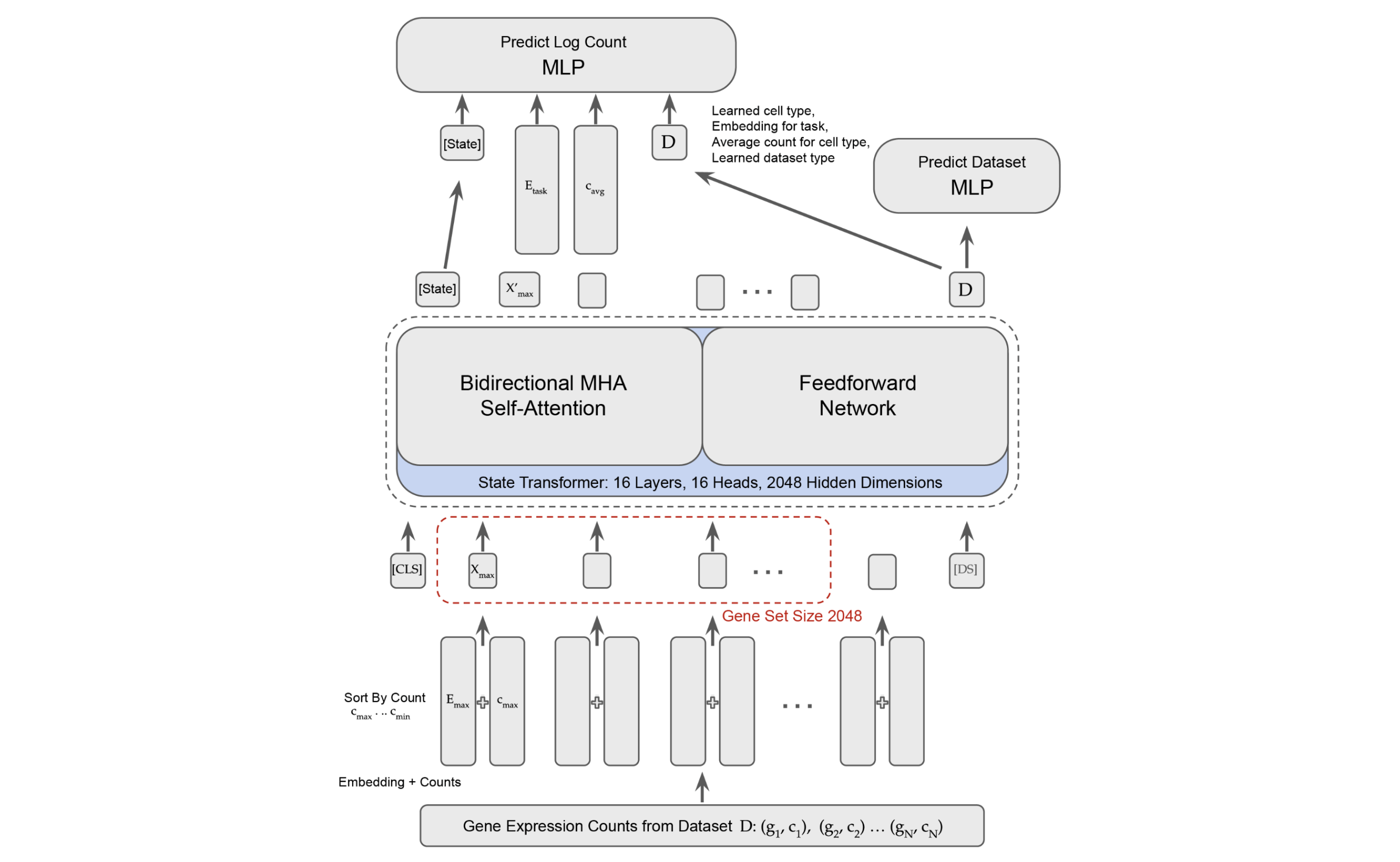
We've now obtained a gene embedding, but what we really want is a cell embedding. To do this, Arc represents each cell as the top 2048 genes ranked by log fold expression level.

We then construct a "cell sentence" from our 2048 gene embeddings as follows:

$$\tilde{\mathbf{c}}^{(i)} = \left[\mathbf{z}_{\text{cls}}, \tilde{\mathbf{g}}_1^{(i)}, \tilde{\mathbf{g}}_2^{(i)}, \ldots, \tilde{\mathbf{g}}_L^{(i)}, \mathbf{z}_{\text{ds}}\right] \in \mathbb{R}^{(L+2) \times h}$$

We add a $\texttt{[CLS]}$ token and $\texttt{[DS]}$ token to our sentence. The $\texttt{[CLS]}$ token ends up being used as our "cell embedding" (very BERT-like) and the $\texttt{[DS]}$ token is used to "disentangle dataset-specific effects". Although the genes are sorted by log fold expression level, Arc further enforces the magnitude of each genes expression by incorporating the transcriptome in a fashion analogous to positional embeddings. Through an odd "soft binning" algorithm and 2 MLPs, they create some "expression encodings" which they then add to each gene embedding. This should modulate the magnitude of each gene embedding by how intensely it is expressed in the transcriptome.

To train the model, they mask 1280 genes per cell, and the model is tasked with predicting them. The 1280 genes are selected such that they have a wide range of expression intensities. For the graphically inclined, the below demonstrates the construction of the cell sentence.

Evaluations 

Understanding how your submission will be evaluated is key to success. The 3 evaluation metrics chosen by Arc are Perturbation Discrimination, Differential Expression and Mean Average Error. Given that Mean Average Error is simple and exactly as it sounds, we will omit it from our analysis.

Perturbation Discrimination

Perturbation Discrimination intends to evaluate how well your model can uncover relative differences between perturbations. To do this, we compute the Manhattan distances for all the measured perturbed transcriptomes in the test set (the ground truth we are trying to predict, $y_t$ and all other perturbed transcriptomes, $y_p^n$) to our predicted transcriptome $\hat{y}_t$. We then rank where the ground truth lands with respect to all transcriptomes as follows:

$$r_t = \sum_{p \neq t} \mathbf{1}\{d(\hat{y}_t, y_p) < d(\hat{y}_t, y_t)\}$$

After, we normalize by the total number of transcriptomes:

$$\text{PDisc}_t = \frac{r_t}{T}$$

Where $0$ would be a perfect match. The overall score for your predictions is the mean of all $\text{PDisc}_t$. This is then normalized to:

$$\text{PDiscNorm} = 1 - 2\text{PDisc}$$

We multiply by 2 as for a random prediction, ~half of the results would be closer and half would be further away.

Differential Expression

Differential Expression intends to evaluate what fraction of the truly affected genes did you correctly identify as significantly affected. Firstly, for each gene compute a $p$-value using a Wilcoxon rank-sum test with tie correction. We do this for both our predicted perturbation distribution and the ground truth perturbation distribution.

Next, we apply the Benjamini-Hochberg procedure, basically some stats to modulate the $p$-values, as with $20,000$ genes and a $p$-value threshold of $0.05$, you'd expect $1,000$ false positives. We denote our set of predicted differentially expressed genes $G_{p,pred}$, and the ground truth set of differentially expressed genes $G_{p,true}$.

If the size of our set is less than the ground truth set size, take the intersection of the sets, and divide by the true number of differentially expressed genes as follows:

$$DE_p = \frac{G_{p,pred} \cap G_{p,true}}{n_{p,true}}$$

If the size of our set is greater than the ground truth set size, select the subset we predict are most differentially expressed (our "most confident" predictions, denoted $\tilde{G}_{p,pred}$), take the intersection with the ground truth set, and then divide by the true number.

$$DE_p = \frac{\tilde{G}_{p,pred} \cap G_{p,true}}{n_{p,true}}$$

Do this for all predicted perturbations and take the mean to obtain the final score.

Conclusion

If a virtual cell can accurately model the change in a cells state in response to perturbations, we can look forward to a very interesting time in pharma. I hope this post accelerated your understanding of the challenge.

May the best team win.

@online{christopherfleetwood2025,
  author = {Christopher Fleetwood},
  title = {Arc Virtual Cell Challenge: A Primer},
  date = {2025-07-05},
  url = {https://fleetwood.dev/posts/virtual-cell-challenge},
  urldate = {2025-07-05}
}