In order to perform classification on a functional brain scan it first undergoes many preprocessing steps. One of these steps is the transformation from the timeseries output of the fMRI scan, transforming a (where is the number of timepoints recorded and is the number of brain regions used) to an matrix of similiarity values (called a connectome). This similarity value is a measure of the neural synchronization between the 2 regions.
So how do we quantify the similarity of 2 different timeseries? This blog post will explore the common ways of quantifying time series similarity in a neuroscientific setting. Before we get into the actual methods used to calculate time series similarity, we need to cover the corner stone of almost all of the methods we are about to explore - covariance.
Covariance
Covariance is simply a measure of how two random variables change together. Below is the formula for calculating covariance:
In the case of fMRI, we have a multivariate random variable, allowing us to use Maximum Likelihood Estimation to estimate the covariance matrix. Below is a toy example of our estimated covariance matrix.
This estimated covariance matrix is called the empirical covariance matrix. In practice we don't use the covariance matrix for our fMRI analyis. This for a number of reasons:
- Covariance is bound between and making it less suitable for downstream classifiers.
- Covariance coefficients are not standardized and cannot be used to quantify the strength of the relationship.
- Symmetric Positive semi-definite (SPD) matricies do not naturally form a Euclidean space (this will be important later).
- When the number of features is large relative to the number of observations, the sample/empirical covariance matrix has excessive estimation error.
Many of the following approaches will aim to address some or all of the above drawbacks with empirical covariance.
To address the excessive estimation error, it is common to perform a transformation to the covariance coefficients, known as "shrinkage". In their seminal paper, "Honey, I shrunk the Sample Covariance Matrix" [1], Ledoit & Wolf proposed using shrinkage to regularize the sample covariance matrix. "Shrinkage" as the name implies, pulls the most extreme covariance coefficients towards more central values. This not only resolves our excessive estimation error, it can also make the matrix easily invertable by encouraging numerical stability. (The interested reader should consult the scikit-learn docs [2] )
Now that we have a well conditioned covariance matrix, we can attempt to address some of the other identified drawbacks.
Canonical Approaches
Pearson's correlation coefficient (Pearson's ) or simply correlation, is the most commonly used method to quantify similarity between 2 fMRI timeseries. Correlation is a linear metric computed from the covariance of the 2 timeseries. Below is the mathematical formula to compute correlation for a pair of random variables:
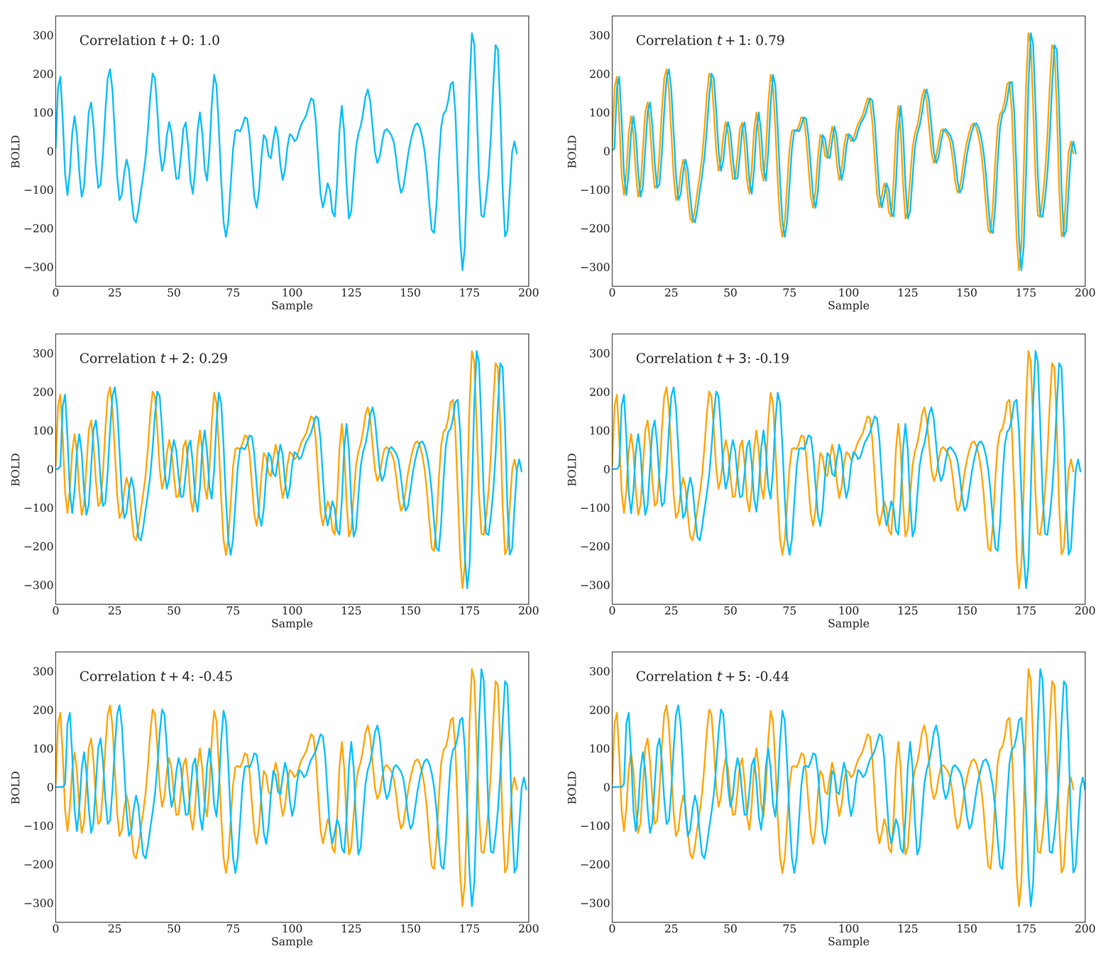
Correlation is widely used in neuroscience as it has long statistical history and is bound between -1 and 1. However, correlation does have some disadvantages. The below figure should demonstrate one clearly:

Due to correlations linear nature, the same timeseries being slightly out of phase causes a huge decrease in the correlation value. Additionally, correlation provides no distinction between whether 2 regions are directly connected or indirectly connected via another region. To account for this, we can use partial correlation!
Partial correlation is a variant of PCC that attempts to address distinguishing between direct and indirect connections. This is done by computing correlation between regions after regressing all other timeseries. Partial correlation is computed from the inverse of the covariance matrix (this is where the shrinkage comes in handy), also known as the precision matrix. Below is the mathematical formula for computing partial correlation for a pair of random variables:
where is the respective precision matrix (obtained through inversion of our well conditioned covariance matrix).
Novel Approaches
Tangent space parameterization is a recently proposed solution to the problematic nature of SPD matricies, in that they don't naturally form Euclidean spaces. Varoquax et al. [3] proposed a solution to this sticky problem. Whilst I won't profess to be an expert on differential manifolds or Riemmenian geometry, here is how I understand it.
Any covariance matrix is a symmetric positive semi-definite matrix. In order to preserve the geometry during our transformations, we need to perform a projection into a space where our geometry is preserved. As SPD matricies form a diffentiable manifold, we can use this fact and Riemannian geometry to keep our geometric intutions in tact.

Image source
The above image makes it clear that if we perform Euclidean operations like subtraction in our manifold, the distances and therefore the geometry will break down. By defining a homomorphic (ie structure preserving) tangent space, we can approximate the distance on the manifold using Euclidean distance in the tangent space!
But we aren't quite out of the woods yet, since we still need to define the reference point on the manifold. As all of our covariance matricies need to be projected into the same tangent space, we need to choose an appropriate reference point. To do this, Varoquax et al. compute the geometric mean of the matricies to define a reference space.
In their paper, Dadi et al. [4] showed that across many fMRI classification tasks, tangent space parameterization should be preferred over both correlation and partial correlation.
Dynamic Time Warping (DTW) is not like the previously discussed methods, as it does not rely on covariance matricies. DTW is one of the canonical algorithms used for measuring similarity between timeseries. It is commonly used in scenarios where timeseries may have a different length or be temporally offest. DTW is a non linear metric, and calculates the optimal match between two given sequences with certain restrictions.
DTW was first proposed for usage with fMRI timeseries by Meszlényi et al. [5]. They propose its value for fMRI timeseries analysis as it has been noted that "dynamic switch of brain states" can cause non-stationary time lags. If there are known or unknown mechanisms in the brain that cause regional time differences in hemodynamic response - DTW could be a great way to account for this.
Below is a Rust implementation of windowed DTW. The window refers to the maximal warping distance.
let m = s.len() + 1;
let n = t.len() + 1;
let mut dtw = Array::from_elem((m, n), f64::MAX);

dtw[[0, 0]] = 0.;

let max_window = i32::max(*window, i32::abs((n - m) as i32));
for si in 1..n {
    let lower_bound = i32::max(1, si as i32 - max_window);
    let upper_bound = i32::min(m as i32, si as i32 + max_window);
    for ti in lower_bound as usize..upper_bound as usize {
        let cost = distance_fn(&s[si - 1], &t[ti - 1]);
        dtw[[si, ti]] = cost +
            f64::min(
                f64::min(dtw[[si - 1, ti]], dtw[[si, ti - 1]]),
                dtw[[si - 1, ti - 1]]
            );
    }
}
Dynamic Time Warping does have some disadvantages. One particularly troublesome one being the computational complexity - . The paper from Meszlényi et al. does come with a DTW implementation for fMRI data on GitHub, however it is extremely cumbersome and difficult to get running (particularly on HPC systems where you don't have root access.)
To address this I wrote RustDTW, a Python module backed by Rust code that works natively within Python on numpy matricies. Check out an example of using DTW for fMRI classification here. My basic testing shows that it should be nearly 10x faster than a mutlithreaded Python implementation.
Classification Performance
Whilst not meant to be an exhaustive exploration of the different connectivity metrics explored above (and itself is not an exhaustive exploration of available connectivity metrics, for more please see Pervaiz et al. [6] I thought I would demonstrate a comparison between them using a large open source dataset. You can check out the inner workings and run it for yourself on Colab here!
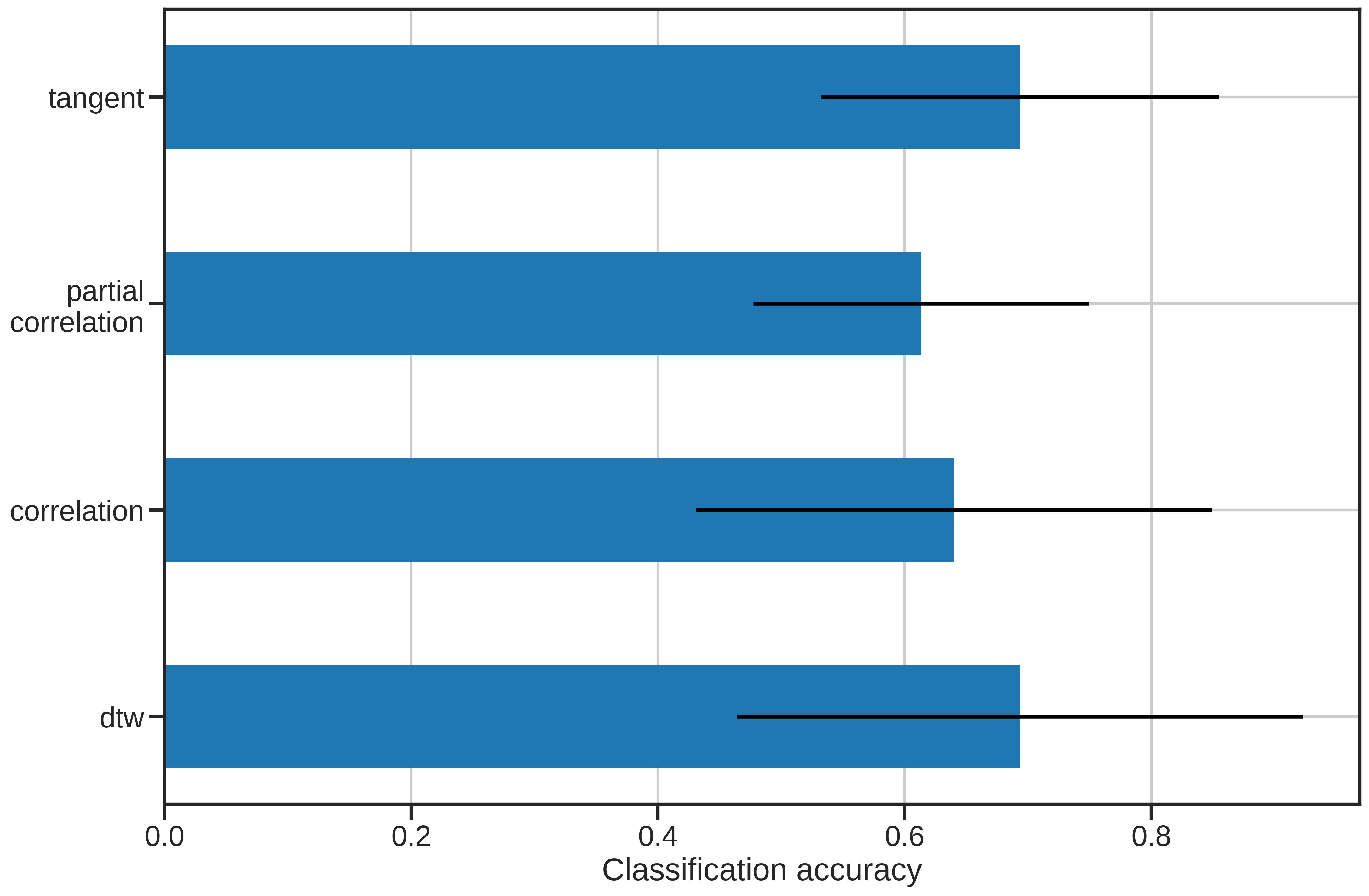
For those just interested in the results, the below graph summarizes the performance of each of the similarity metrics.

The results are pretty interesting! We can see that both non-linear matching and transforming the covariance matricies into a natural space can provide improvements over standard correlation. Perhaps a future metric will incorporate characteristics from both tangent space parameterization and DTW to improve performance.